Notes
Before gathering data:
- Choose image size (critical)
- Choose expectation (percentage)
- Build dataset
- Training set
- Validation set
- Test set
- Resize image temporarily
- Review dataset with small image size
Probability
(Give us a formal way of reasoning about the level of certainty)
Basic probability theory
Natural approach to measure probability: Take an individual times for a value and divide it by total number of times
Law of large number: Having more experimenting times, the probabilities will come closer and closer to the underlying probabilities
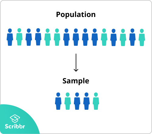
Sampling: Draw examples from probability distributions
Multinomial distribution (Phân phối đa thức): The distribution that assigns probabilities to a number of discrete choices
Axioms of Probability Theory
- Sample space or outcome space: Total results, samples or outcomes of a problem.
F.e: When rolling a dice, we have a sample space of $S = {1, 2, 3, 4, 5, 6}$
- Event: A set of outcomes from a given sample space.
F.e: An event of getting an odd number when rolling a dice.
- The probability of an event A in the given sample space S is denoted as P(A), satisfies the following properties:
- $P(A) ≥ 0$
- $P(S) = 1$
- For mutually exclusive events, the probability that any happens = sum of their individual probabilities
Random variables (Biến ngẫu nhiên):
Set X as a random variable, rather than specifying accurate like P(X = a), we can illustrate:
- $P(X)$ as the distribution over the random variable X
- $P(a)$ as a probability of a specific value
There is a difference between discrete and continuous random variables.
- Discrete RV: Numerical values
- Continuous RV: Infinite amount of values
F.e: Assume we calculate the probability of a person having height = 1.8m. If we take precise measurements, that height might be 1.80139278291028719, and no one else can have that height. So it is reasonable that we use interval for calculating the probabilities, like height of people falling between 1.7-1.8m
2.6.2 Dealing with multiple Random Variables:
Very often, we will want to consider more than one random variable at a time. For instance, we may want to model the relationship between diseases and symptoms. Given a disease and a symptom, say “flu” and “cough”, either may or may not occur in a patient with some probability. While we hope that the probability of both would be close to zero, we may want to estimate these probabilities and their relationships to each other so that we may apply our inferences to effect better medical care.
As a more complicated example, images contain millions of pixels, thus millions of random variables. And in many cases images will come with a label, identifying objects in the image. We can also think of the label as a random variable. We can even think of all the metadata as random variables such as location, time, aperture, focal length, ISO, focus distance, and camera type. All of these are random variables that occur jointly. When we deal with multiple random variables, there are several quantities of interest.
Joint probability: Two events have to happen simultaneously.
Notation: \(P(A = a, B = b) ~~or~~ P(A ∩ B)\)
Note: \(P(A ∩ B) ≤ P(A), P(B)\)
Conditional probability: Probability of B = b, provided that A = a has occurred.
| Notation and formula: $$P(B=b | A=a) = \frac{P(B = b, A = a)}{P(A = a)} = \frac{P(A ~∩~ B)}{P(A = a)}$$ |
Bayes’ Theorem:
\[P(A | B) = \frac{P(B | A) . P(A)}{P(B)} (1)\]| To be more clear: Because $$P(A ∩ B) = P(B | A) . P(A) = P(A | B) . P(B)$$ |
→ (1) is true
Marginalization (Phép biên hóa):
Operation of determining $P(B)$ from $P(A, B)$. To be more theoretically:
Marginalisation is a method that requires summing over the possible values of one variable to determine the marginal contribution of another.
which is also known as sum rule. The probability or distribution of marginalization is called a marginal probability or marginal distribution
Formulation: \(P(B) = AP(A, B)\)
Independence:
Two independent variables: The occurrence of an event A does not reveal any information of the occurrence of an event B
| → P(B | A) = P(B) → P(A, B) = P(A) * P(B) |
Two events are independent only when the probability of their joint distribution is equal to the product of the individual probabilities
2.6.3 Expectation and variance:
Expectation and variance offer useful measures to summarize key characteristics of probability distributions
Expectation (average) of random variable X:
Formula: \(E[X] = xx P (X=x)\)
Variance:
Measure how much the random variable X deviates from its expectation
Formula: \(Var[X] = E [(X − E[X])2] = E[X2] − E[X]2\)
Linear Algebra
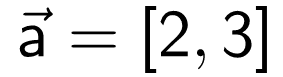
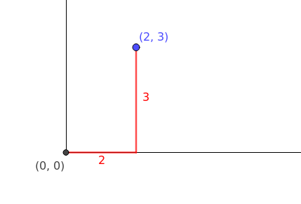
Vectors
Definition
Vectors are 1-dimensional arrays of numbers or terms. In geometry, vectors store the magnitude and direction of a potential change to a point (The vector [3, -2] says go right 3 and down 2)
Notation
\[v = \begin{bmatrix}1 \\ 2 \\ 3 \end{bmatrix}\]Vectors in geometry
Operations
Scalar operation: $\begin{bmatrix} 2
2
2
\end{bmatrix} + 1 = \begin{bmatrix} 3
3
3
\end{bmatrix}$
Element-wise operation: $\begin{bmatrix} a_1
a_2
\end{bmatrix} + \begin{bmatrix} b_1
b_2
\end{bmatrix} = \begin{bmatrix} a_1+b_1
a_2+b_2
\end{bmatrix}$
Dot product: $\begin{bmatrix} a_1
a_2
\end{bmatrix} \cdot \begin{bmatrix} b_1
b_2
\end{bmatrix} = a_1 b_1+a_2 b_2$
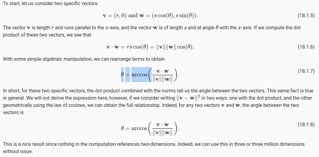
Angle of dot product:
Hadamard product (elementwise multiplication): \(\begin{bmatrix} a_1 \\ a_2 \\ \end{bmatrix} \odot \begin{bmatrix} b_1 \\ b_2 \\ \end{bmatrix} = \begin{bmatrix} a_1 \cdot b_1 \\ a_2 \cdot b_2 \\ \end{bmatrix}\)
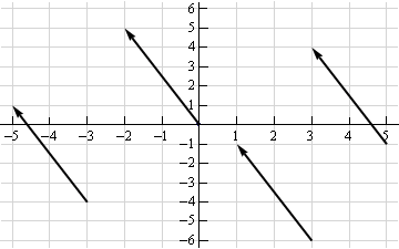
Vector fields
A vector field shows how far the point (x,y) would hypothetically move if we applied a vector function to it like addition or multiplication
Matrices
Dimensions
\[\begin{bmatrix} 2 & 4 \\ 5 & -7 \\ 12 & 5 \\ \end{bmatrix} \begin{bmatrix} a² & 2a & 8\\ 18 & 7a-4 & 10\\ \end{bmatrix}\]1 has dimensions (3, 2)
2 has dimension (2, 3)
Operations
Scalar operation: $\begin{bmatrix} 2 & 3
2 & 3
2 & 3
\end{bmatrix} + 1 = \begin{bmatrix} 3 & 4
3 & 4
3 & 4
\end{bmatrix}$
Elementwise operation: $\begin{bmatrix} a & b
c & d
\end{bmatrix} + \begin{bmatrix} 1 & 2
3 & 4
\end{bmatrix} = \begin{bmatrix} a+1 & b+2
c+3 & d+4
\end{bmatrix}$
Hadamard product:
- $\begin{bmatrix} a_1 & a_2
a_3 & a_4
\end{bmatrix} \odot \begin{bmatrix} b_1 & b_2
b_3 & b_4
\end{bmatrix} = \begin{bmatrix} a_1 \cdot b_1 & a_2 \cdot b_2
a_3 \cdot b_3 & a_4 \cdot b_4
\end{bmatrix}$ - $\begin{bmatrix} {a_1}
{a_2}
\end{bmatrix} \odot \begin{bmatrix} b_1 & b_2
b_3 & b_4
\end{bmatrix} = \begin{bmatrix} a_1 \cdot b_1 & a_1 \cdot b_2
a_2 \cdot b_3 & a_2 \cdot b_4
\end{bmatrix}$
Matrix transpose: $\begin{bmatrix} a & b
c & d
e & f
\end{bmatrix} \quad \Rightarrow \quad \begin{bmatrix} a & c & e
b & d & f
\end{bmatrix}$
Matrix multiplication: $\begin{bmatrix} a & b
c & d
e & f
\end{bmatrix} \cdot \begin{bmatrix} 1 & 2
3 & 4
\end{bmatrix} = \begin{bmatrix} 1a + 3b & 2a + 4b
1c + 3d & 2c + 4d
1e + 3f & 2e + 4f
\end{bmatrix}$
Norms
Definition
It is a function that returns length/size of any vector
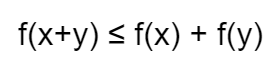
Conditions
Condition 1

Condition 2
Condition 3
Usual norms
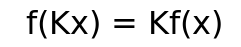
- 1-Norm (Manhattan Distance):
| $ | a | _1 = (2 + 3)^1$ |
2-Norm (L2 distance): $ \mathbf{x} _2 = \sqrt{x_1^2 + x_2^2 + \dots x_n^2}$ p-Norm (p ≥ 1): $ \mathbf{x} _p = ( x_1 ^p + x_2 ^p + \dots x_n ^p)^{\frac{1}{p}}$
Cosine similarity
Measure the closeness of two vectors. Value ranges from [-1; 1]
Formula: $\cos(\theta) = \frac{\mathbf{v}\cdot\mathbf{w}}{|\mathbf{v}||\mathbf{w}|}$
Linear Dependence, Linear Independence, and Rank
Cho một hệ gồm m vector $(v_1, v_2, …, v_n)$
Tổ hợp tuyến tính: $\alpha_1.v_1 + \alpha_2.v_2 + … + \alpha_3.v_3 = \vec{0} ~~ (1)$
⇒ Các vector này là độc lập tuyến tính khi và chỉ khi $\alpha_1 = \alpha_2 = … = \alpha_n = 0$ để thỏa mãn $(1)$
⇒ Các vector này là phụ thuộc tuyến tính khi $\exists \alpha_i \ne 0$ để thỏa mãn $(1)$
⇒ Hạng của ma trận là số lượng vector độc lập tuyến tính trong ma trận đó